Academic Signal #5

Position-sizing with the Kelly criterion (how it works in the real world)

New Columbia research reveals that textbook Kelly formulas systematically overestimate optimal position sizes when you account for actual market behavior.

Most Kelly Criterion applications in finance rely on plugging theoretical parameters (expected excess return μ, variance σ²) into the standard formula f* = μ/σ². This Columbia research optimizes position-sizing based on actual historical data, taking into account the messiness of markets (such as fat tails and discrete rebalancing periods).

The result? Running the optimizer on actual return series trims the S&P 500 Kelly fraction from 2.32x with daily rebalancing down to 1.80x when you rebalance annually, and it falls further to 1.47x over the crash‑heavy 1926‑84 window (a 22‑36 % haircut versus the textbook formula).

Kelly Criterion 101: The Math That Matters

The Kelly formula determines the optimal fraction of your portfolio to risk on any given bet to maximize long-term wealth growth.

f* = (bp - q) / b

Where:

• f* = fraction of your bankroll to bet

• b = odds received (how much you win per $1 bet)

• p = probability of winning

• q = probability of losing (1-p)

Simple example: You find a biased coin that lands heads 60% of the time. A casino offers even money bets (win $1 for every $1 bet). How much of your bankroll should you bet?

• p = 0.60 (60% chance of winning)

• q = 0.40 (40% chance of losing)

• b = 1 (win $1 for every $1 bet)

Kelly formula: f* = (1×0.60 - 0.40) / 1 = 0.20 = 20%

Why does 20% make sense? You have a real edge (winning 60% vs. the 50% needed to break even), but you can still lose each individual bet. Betting 20% means:

• You're aggressive enough to capitalize on your 10-percentage-point edge

• You're conservative enough that even a string of losses won't wipe you out

• If you bet less (say 10%), you're not making enough from your edge

• If you bet more (say 40%), you risk going broke during inevitable losing streaks

What is the Kelly formula optimizing? It maximizes the geometric mean return (compound annual growth rate) of your wealth over time. It's NOT maximizing your arithmetic average return, Sharpe ratio, or minimizing risk.

For investing, the Kelly formula becomes: f* = μ / σ²

Where:

• μ = expected excess return above risk-free rate (typically 3-month Treasury bills)

• σ² = variance of returns

🤔 How does the gambling formula become the investing formula? Conceptually, they're the same thing applied to different situations:

Gambling version: f* = (bp - q) / b

• (bp - q) = your "edge" per unit bet

• b = the odds structure/risk you face

Investing version: f* = μ / σ²

• μ = your "edge" over risk-free returns

• σ² = the uncertainty/risk you face

The transformation happens when you move from discrete win/lose outcomes to continuous return distributions. When you assume stock returns follow a normal distribution and use calculus to maximize expected logarithmic growth, the gambling formula mathematically becomes the investing formula.

Both are saying the same thing: bet more when you have a bigger edge, bet less when there's more uncertainty.

What the Data Actually Shows

The researchers tested their approach across multiple time periods and assets, revealing patterns that should change how you think about Kelly calculations:

S&P 500 Optimal Kelly Leverage by Period:

• 1997-2024 (daily rebalancing): 2.4x

• 1926-2024 (daily rebalancing): 2.32x

• 1926-2024 (annual rebalancing): 1.8x

• 1926-1984 (annual rebalancing): 1.47x

• 1985-2024 (annual rebalancing): 2.2x

Three critical patterns emerge:

1. Crisis periods matter: The 1926-1984 period (including Great Depression) suggests only 1.47x leverage, while 1985-2024 suggests 2.2x. Including major historical crises systematically reduces optimal leverage because the fat tail risk is much higher than normal (aka ‘Gaussian’) distributions assume.

Because Kelly maximizes expected log wealth (that is, it chooses the position size that maximizes the expected value of the logarithm of your wealth, which is equivalent to maximizing long-run geometric growth), those rare deep losses carry an outsized penalty, so the growth‑optimal Kelly fraction falls when you estimate it from real return series with crashes.

2. Rebalancing frequency is crucial: Daily rebalancing allows ~30% higher leverage (2.32x vs 1.8x for the same period) because you can respond to market moves quickly. 

When you rebalance less often, returns arrive in lumpier, more left‑tailed chunks, and leverage drifts upward after losses, so the expected‑growth‑maximizing Kelly fraction drops as you move from daily toward annual rebalancing.

But this only works if you actually rebalance daily – using daily data to size a quarterly rebalanced position is dangerous.

Daily rebalancing example: You start with $100k and 2.0x leverage ($200k invested). Market drops 20% → your position is now worth $160k, but your equity is only $60k → your leverage has drifted to 2.67x (dangerously high). Daily rebalancing forces you to sell down to $120k invested (2.0x of your new $60k equity), protecting you from excessive leverage during drawdowns.

Annual rebalancing: You're stuck at 2.67x leverage for potentially months. If the market drops another 20%, your 2.67x leverage means you lose 53% of your remaining equity. You could face margin calls or complete ruin before you get to rebalance.

The key insight: "Responding to market moves" isn't about timing or predicting markets - it's about maintaining constant optimal risk exposure. Daily rebalancing prevents leverage from drifting to dangerous levels during losing streaks, while also preventing it from becoming too conservative during winning streaks. You're managing risk more actively, so you can take on more leverage.

3. Time horizon interpretation: Should you use the longest time horizon available? Yes, but with important caveats. Longer periods give you more data on tail events, but they also include market regimes that may not be relevant today. The research suggests including at least one major crisis period in your calculations, even if it's decades old.

Practical implication: If you're managing institutional money, use the longest available dataset that includes major market dislocations. The Great Depression data might seem ancient, but it captures tail risk that more recent periods miss. Your Kelly calculations should reflect worst-case scenarios, not just average market conditions.

Multi-Asset Kelly: Where It Gets Really Interesting

The key insight: proper diversification doesn't just reduce risk – it allows for optimal leverage on each individual position.

Two-Asset Results:

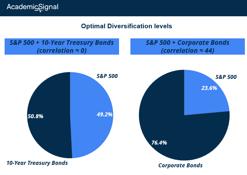
S&P 500 + 10-Year Treasury Bonds (correlation ≈ 0):

• Optimal allocation: 1.58x stocks, 1.63x bonds

• Total leverage: ~3.2x

• Compare to single-asset Kelly: 1.67x stocks, 2.42x bonds

S&P 500 + Corporate Bonds (correlation 0.44):

• Optimal allocation: 0.83x stocks, 2.69x bonds

• Total leverage: ~3.5x

• The higher correlation reduces stock allocation, but corporate bonds' superior risk-return profile gets high leverage

Why multi-asset Kelly works better:

1. Diversification dividend: Uncorrelated assets let you take more risk in each position because portfolio-level volatility is lower

2. Correlation matters a lot: Near-zero correlation (stocks/Treasuries) allows high leverage in both. Higher correlation (stocks/corporate bonds) requires rebalancing between assets

3. Risk-adjusted returns drive allocation: Corporate bonds got 2.69x leverage because their Sharpe ratio was superior to stocks over this period

Three-Asset Constraints: When the researchers added Treasury bonds to the S&P 500/corporate bond portfolio with individual leverage limits of 1.7x, the optimizer allocated: 1.16x stocks, 0.63x Treasuries, 1.70x corporate bonds.

This shows that Kelly isn't just about position sizing - it's about optimal portfolio construction where the math tells you how much diversification benefit you're actually getting.

The Bottom Line

For Portfolio Managers: If you're using Kelly-based position sizing, three changes matter:

1. Use actual return data instead of theoretical assumptions

2. Account for your actual rebalancing frequency

3. Add practical constraints like maximum drawdowns

For Risk Management: The research provides mathematical backing for fractional Kelly approaches. Half-Kelly delivers ~85% of the growth benefits with dramatically lower volatility.

For Asset Allocation: Multi-asset Kelly optimization isn't just about diversification - it's about finding combinations that allow higher leverage per asset while maintaining portfolio-level risk constraints.

The key insight: Kelly Criterion works, but only when you feed it realistic inputs and constraints. The theoretical versions taught in textbooks systematically overestimate optimal leverage because they ignore the messy realities of actual market behavior.

POLL